Introduction⌗

Frequency-Modulated Continuous-Wave (FMCW) radar is a type of radar sensor capable of determining the target distance and speed by comparing the transmitted signal with the one reflected.

In a nutshell, the radar processor performs two consecutive Fast Fourier Transform (FFT) over the received signal to compute the range-Doppler map of the illuminated area. After a square-law detector, each range-Doppler map cell represents the presence of a potential target lying at the corresponding cell range and Doppler frequency which can be used to estimate its speed. If the cell value is greater than a threshold (computed to ensure a constant Probability of False Alarm) a target is detected at that cell.

In modern systems, it is often required not only to detect a target but to automatically classify it. To this end, several approaches have been developed using multiple radar features such as the target micro-Doppler signature. However, in this post, we will explore the use of a Convolutional Neural Network (CNN) to classify targets using only the information provided by the range-Doppler map.

You can find the complete code for this post here:

https://github.com/trujilloRJ/fmcw_radar_cnn

Dataset⌗

We will use the Real Doppler RAD-DAR database available in Kaggle at:

https://www.kaggle.com/datasets/iroldan/real-doppler-raddar-database

Additional details about the radar system and the acquisition and labeling process can be found in the original paper at:

https://digital-library.theiet.org/content/journals/10.1049/iet-rsn.2019.0307

The dataset contains 11x61 matrices representing the range-Doppler map cells surrounding a detected target. Three classes are represented in the dataset: Drones, Cars, and People. Hence, our purpose is to train a CNN that accurately classify the target into one of the three classes based on the 11x61 range-Doppler cells matrix.

Data exploration⌗

1. Loading data⌗

First, we need to load the data. The dataset is divided into folders that contain the matrices corresponding to each class stored as .csv files.

Python Loading data


import os
import numpy as np
import pandas as pd
import matplotlib.pyplot as plt

DIR = os.path.abspath('./dataset')
LABEL_MAPPER = {'Cars': 0, 'Drones': 1, 'People': 2}
INV_LABEL_MAPPER = {v: k for k, v in LABEL_MAPPER.items()}
DEVICE = torch.device('cuda:0' if torch.cuda.is_available() else 'cpu')

def get_data_for_label(label: str):
X, y = [], []
for root, dirs, files in os.walk(os.path.join(DIR, label)):
for file in files:
if file.endswith('.csv'):
y.append(LABEL_MAPPER[label])
df = pd.read_csv(os.path.join(root, file), sep=',', header=None)
X.append(df.values)
print(f'Loaded {len(y)} examples for label {label} encoded with {LABEL_MAPPER[label]}')
return X, y

X_cars, y_cars = get_data_for_label('Cars')
X_drones, y_drones = get_data_for_label('Drones')
X_people, y_people = get_data_for_label('People')

X = X_cars + X_drones + X_people
y = y_cars + y_drones + y_people
X, y = np.array(X), np.array(y)

In the above code, after loading the data we arranged the feature matrices into X and the encoded classes into y.

2. Data inspection⌗

First, let’s check if the dataset is imbalanced by seeing the number of examples corresponding to each class.

Python


fig, ax = plt.subplots()
ax.bar(['Cars', 'Drones', 'People'], [len(x) for x in [y_cars, y_drones, y_people]])
ax.set_title('Class distribution')

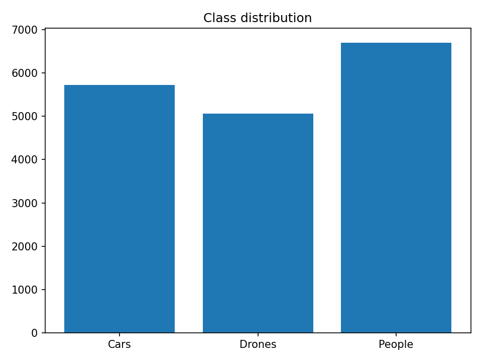
From the figure, there are:

5720 examples of cars
5065 examples of drones
6700 examples of people

For a total of 17485 examples. In addition, all classes are approximately equally represented, hence we don’t need to worry about dataset imbalance. This allows us to safely use the prediction accuracy as a metric to measure our model performance.

Now, let’s visualize individual class examples to see if we can gain more insight into the data.

Python Visualizing data examples


import itertools

fig, axs = plt.subplots(3, 3, figsize=(10, 10))
for i, j in itertools.product(range(3), range(3)):
index = np.random.randint(0, len(y)-1)
img = axs[i, j].imshow(X[index], cmap='jet', vmin=-140, vmax=-70)
axs[i, j].set_title(f'{INV_LABEL_MAPPER[y[index]]}')
axs[i, j].axis('tight')

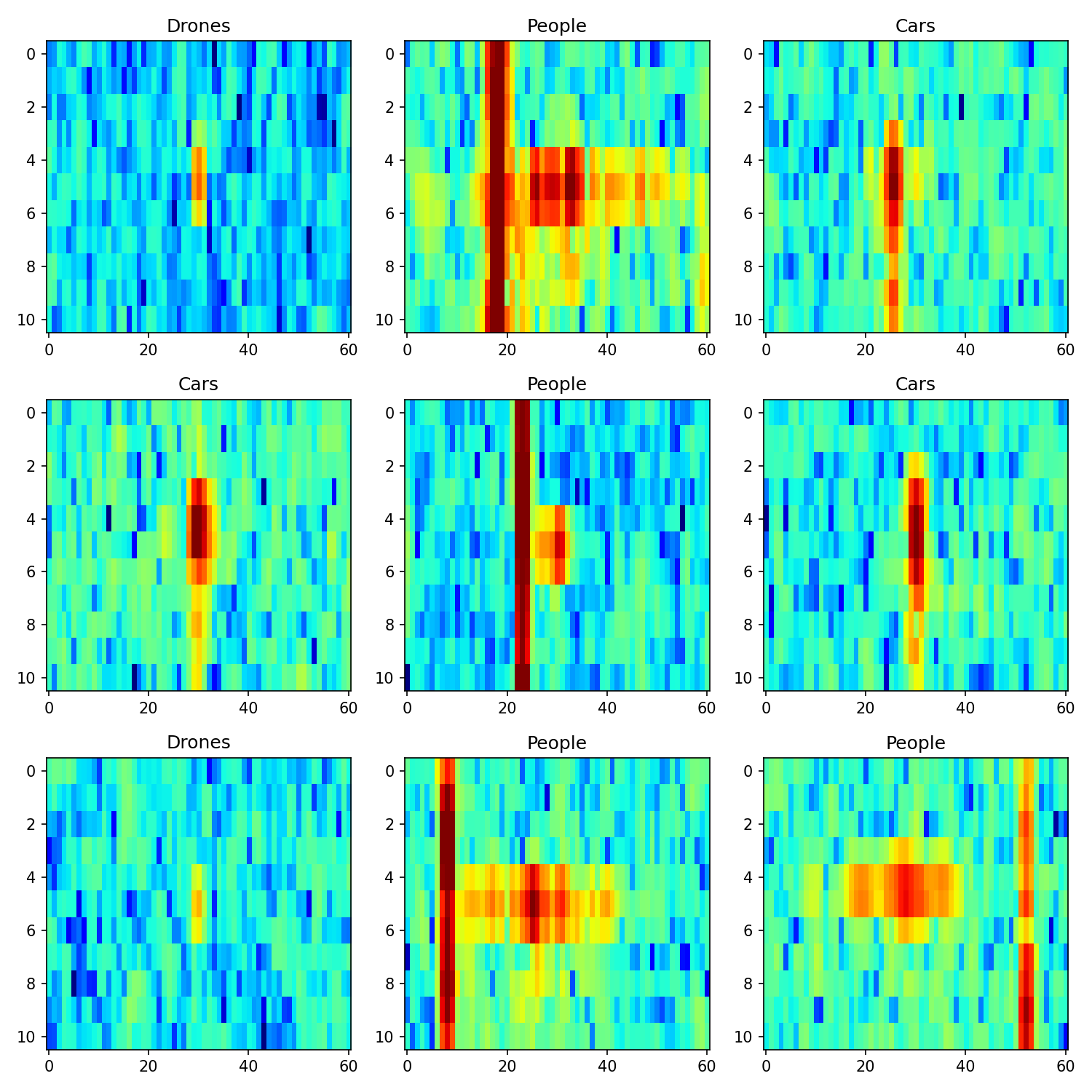
There are a couple of observations that we can make from the previous figure:

Car reflections usually take multiple cells on the y-axis direction which represents the range dimension and few on the x-axis or Doppler dimension. This is expected since cars are large targets with no moving parts.
On the other hand, drone reflections are smaller and have low power values compared to cars and people. This is also expected since drones have the smallest Radar-Cross Section (RCS) of the analyzed targets which is directly proportional to the echo power.
People’s reflections are wild 😬! They spread through the Doppler dimension as we a move lots of parts when walking. Take for example the movement of the arms.
In addition, people’s maps have strong side echoes (represented by a red rectangle) that take the whole range dimension. I suspect that these are clutter echoes corresponding to stationary objects in the environment, as people move relatively slowly, their echoes usually appear near the clutter. In fact, this could serve as an indicator for our model.

Our hope is that the model learns all these differences and correctly classifies the targets!

Training⌗

We will use PyTorch to train and design our model.

1. Creating custom Dataset class⌗

To ease the training process we create our own custom Dataset class. In particular, this integrates well with the PyTorch data loader which enables several features such as automatic batching.

Python Custom dataset


import torch
from torch.utils.data import Dataset, DataLoader

class MapsDataset(Dataset):
def **init**(self, data, labels):
self.data = torch.from_numpy(data)
self.labels = torch.from_numpy(labels)

    def __len__(self):
        return len(self.data)

    def __getitem__(self, index):
        return self.data[index][None, :], self.labels[index]

2. Train-validation-test splitting⌗

Then, we split the dataset into three: training, validation, and test. The training dataset will be used to train our model and update its parameters while the validation data can be used to optimize it. Finally, the test dataset will serve as a final performance measure for our model.

It is important to prevent overfitting and data leakage that we do not take any decision on our model based on the results of the test dataset. This dataset must represent a real application where the model has not seen the examples before, nor for training or optimization.

Finally, we will use 10% of the data for test, 20% for validation, and the remaining 70% for training.

Python Dataset splitting


from sklearn.model_selection import train_test_split

SEED = 0
val_size, test_size = 0.2, 0.1

# train-test split

X_trainval, X_test, y_trainval, y_test = train_test_split(
X, y, test_size=test_size, random_state=SEED, stratify=y
)

# train-validation split

X_train, X_val, y_train, y_val = train_test_split(
X_trainval,
y_trainval,
test_size=val_size / (1 - test_size),
random_state=SEED,
stratify=y_trainval,
)

# using custom DataLoader

train_dataset = MapsDataset(X_train, y_train)
val_dataset = MapsDataset(X_val, y_val)

3. Testing the first CNN⌗

Our first neural network is inspired by the one proposed in the original paper. It has 1 convolutional layer followed by 4 fully connected layers.

Python Conv1Net


import torch.nn as nn

class Conv1Net(nn.Module):
def **init**(self, k1_size=(3, 3)):
super(Conv1Net, self).**init**()

        # convolutional layer
        self.conv1 = nn.Sequential(
            nn.Conv2d(1, 20, kernel_size=k1_size),
            nn.ReLU(),
            nn.MaxPool2d(2, 2),
        )

        # fully connected layers
        self.fc1 = nn.Sequential(nn.Linear(116 * 20, 64), nn.ReLU())
        self.fc2 = nn.Sequential(nn.Linear(64, 64), nn.ReLU())
        self.fc3 = nn.Sequential(nn.Linear(64, 64), nn.ReLU())
        self.fc4 = nn.Sequential(nn.Linear(64, 3), nn.ReLU())
        self.fc_layers = [self.fc1, self.fc2, self.fc3, self.fc4]

    def forward(self, x):
        x = self.conv1(x)
        x = torch.flatten(x, 1)
        for fc in self.fc_layers:
            x = fc(x)
        return x

We train the previous network with the following parameters:

Parameter	Value
Number of epochs	`25`
Learning rate	`2e-4`
Batch size	`32`
Optimizer	`Adam (torch.optim.Adam)`
Loss function	`Cross-entropy (torch.nn.CrossEntropyLoss())`

The training is easily done using the utility function train_model() that can be found in the repo. The results obtained are:

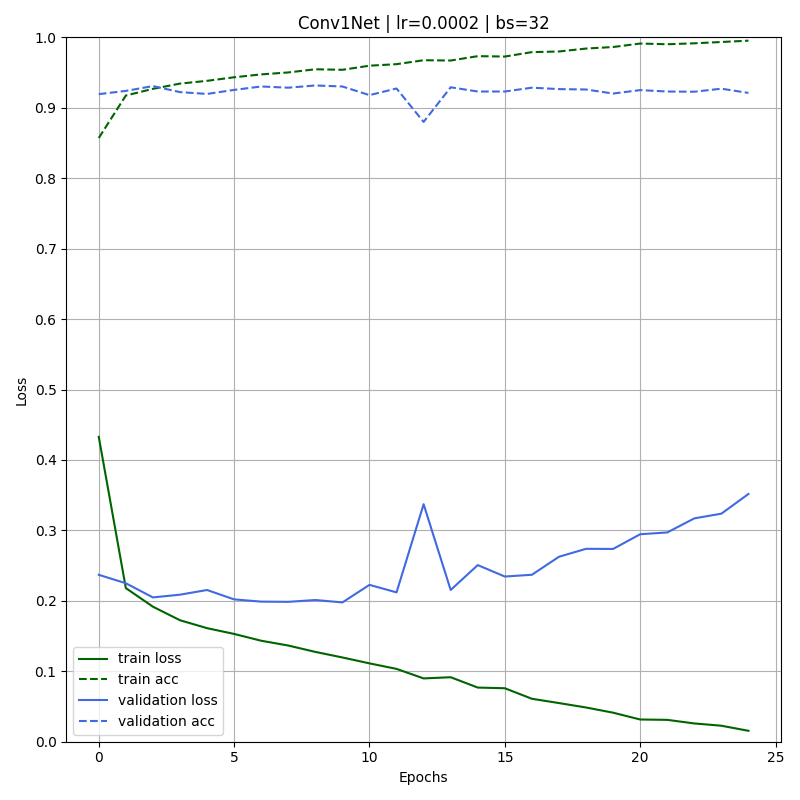
From the figure, we can see that the model starts with high accuracy both for the training and validation set. As the number of epochs increases the training loss reduces while the training accuracy grows. However, the validation loss significantly increases.

In fact, when the training finishes the model presents a performance gap between the training (0.995) and validation (~0.921) accuracy. This is a clear sign that the model is overfitting the data.

Overfitting is a well-known problem in Deep Learning and a number of regularization strategies to reduce it have been proposed such as dropout, early-stopping, and weight regularization among others. Check this article for an exhaustive analysis of regularization techniques: https://arxiv.org/abs/1710.10686

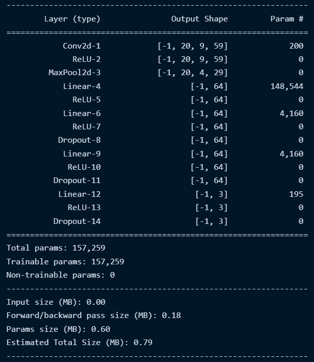
In this post, we will focus on one strategy which is reducing the model complexity. Why? Let’s start by looking at a model summary of Conv1Net

from torchsummary import summary

# here model is Conv1Net instance
summary(model, input_size=(1, 11, 61))

First, we can see that our model has around 157K parameters! This is a lot considering that the number of examples in our data is around 17K. This might suggest that a simpler model could also be able to learn the representations and patterns of the data.
Second, the estimated total size of the model is around 800 KB. Since we are thinking of deploying our net in an FMCW radar system, the memory size could be limited especially if an FPGA-based architecture is used. Therefore, this is an additional motivation to explore a simpler model with fewer parameters.

4. Simplifying the model⌗

The summary shows that the convolutional layers have much fewer parameters than the first three fully connected layers. Since we want to reduce the number of parameters, a basic idea could be to add a convolutional layer while cutting a fully connected one. The new CNN is defined:

Python Conv2Net


class Conv2Net(nn.Module):
def **init**(self, k1_size=(3, 3), k2_size=(3, 3)):
super(Conv2Net, self).**init**()

        # convolutional layers
        self.conv1 = nn.Sequential(
            nn.Conv2d(1, 10, kernel_size=k1_size),
            nn.ReLU(),
            nn.MaxPool2d(2, 2),
        )
        self.conv2 = nn.Sequential(
            nn.Conv2d(10, 20, kernel_size=k2_size),
            nn.ReLU(),
            nn.MaxPool2d(2, 2),
        )

        # fully connected layers
        self.fc1 = nn.Sequential(nn.Linear(20 * 13, 64), nn.ReLU())
        self.fc2 = nn.Sequential(nn.Linear(64, 64), nn.ReLU())
        self.fc3 = nn.Sequential(nn.Linear(64, 3, nn.ReLU()))
        self.fc_layers= [self.fc1, self.fc2, self.fc3]

    def forward(self, x):
        x = self.conv2(self.conv1(x))
        x = torch.flatten(x, 1)
        for fc in self.fc_layers:
            x = fc(x)
        return x

We train the new CNN with the same parameters as before obtaining the following results:

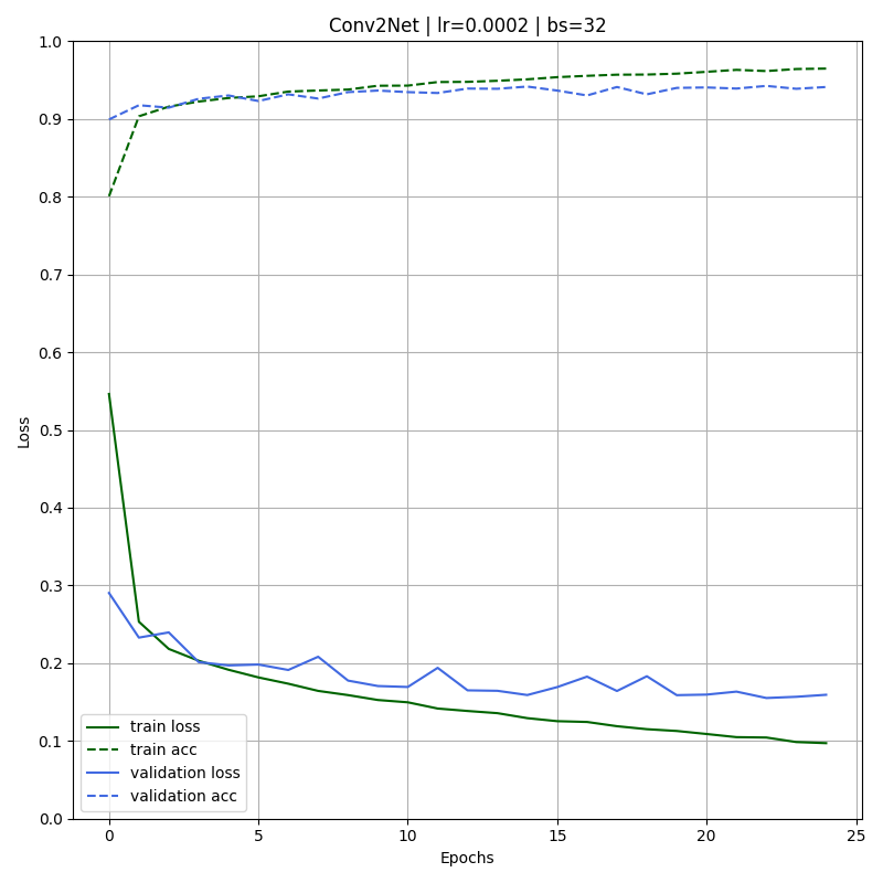
Nice! It can be seen how both training and validation losses decrease on each iteration. Moreover, we have successfully reduced the gap between the training (0.965) and validation (0.941) accuracy. Moreover, the validation accuracy is higher than the one obtained for the first model Conv1Net.

Finally, let’s check the new model summary:

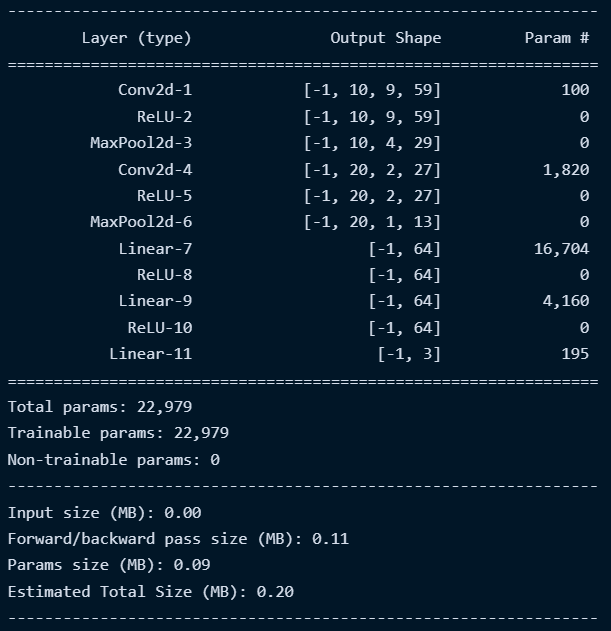
We reduce the number of parameters from 173K to 23K and the model size from 800 KB to 200 KB. All this while improving generalization and obtaining a higher performance on the validation data.

Finally, when applying the model to the test data we obtain a nice: 94 % accuracy.

Conclusions⌗

We trained a CNN for target classification in an FMCW radar system taking as input the range-Doppler map.
We have improved regularization by reducing the model complexity.
The final trained model can achieve an accuracy of about 94 % on unseen data.
We managed to keep the model size to around 200 KB which could be essential for a real-time deployment on FPGA-based architectures.

Future steps and remaining questions⌗

Optimize the model by trying different learning rates, batch sizes, and other hyperparameters. Use learning rate decay?
Extend the training to more epochs. It seems like the model can still learn a little if we increase the number of epochs.
Can we further simplify the model without losing learning capacity?
Try data augmentation techniques such as adding gaussian noise to the maps.
When the model fails? See the worst classification examples.

FMCW radar target classification with a CNN