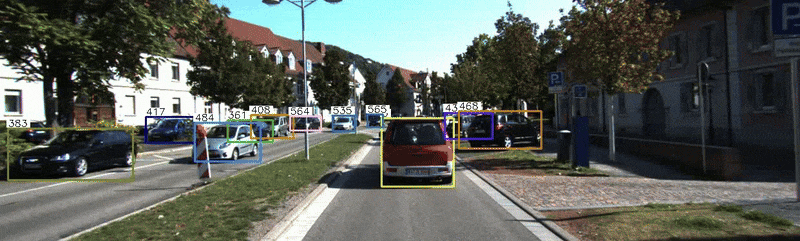
The image above depicts a typical automotive scene captured by a monocular camera at a specific time. The colored boxes represent object detections made by a CNN-based detector, such as YOLO, with each color indicating a different class—green for cars and dark blue for pedestrians. However, these detections are independent across frames since the object detector lacks memory, meaning it does not recognize that an object in one frame is the same in the next.

In automotive applications, detecting objects in isolation is not sufficient. To enable functions like collision avoidance, path planning, and autonomous navigation, it is crucial to consistently identify and track objects as they move through consecutive frames. This process, known as object tracking, assigns a unique identity to each detected object, ensuring continuity and a more comprehensive understanding of the dynamic environment.

In this post, we will explore key concepts of object tracking and present its flow diagram to illustrate the process. Additionally, we will implement a simple yet effective object tracker, widely recognized in the community as the Simple Online and Realtime Tracker (SORT), demonstrating its practical applications to the KITTI object tracking dataset.

Source code⌗

The source code for the object tracker is available at: https://github.com/trujilloRJ/sort_based_object_tracking

Table of Contents⌗

1. System overview
2. State-space model
3. Association stage
4. After association
5. Results
6. Conclusions and next steps

System overview⌗

Let’s begin with an overview of the core steps involved in any tracking system. Later sections will delve deeper into each stage and how SORT specifically implements them.

The following figure illustrates the key stages of a tracking system, which operates on a frame-by-frame basis. Initially, no tracks exist; only detections from the current frame are available. These detections may correspond to real objects or false positives. To account for this uncertainty, the system creates “tentative” tracks for all detections. Over subsequent frames, these tentative tracks are either promoted to established tracks or discarded based on their consistency in being associated with new detections.

Core tracking system diagram.

This method operates under the assumption that false positives are unlikely to persist across multiple frames. However, this introduces a fundamental trade-off: delaying the promotion or removal of tentative tracks enhances precision but slows down track establishment. In automotive applications, this delay can be critical, as rapid responsiveness is essential for safety and performance.

1. Predict tracks next state: Once tracks are created and new frame detections become available, the first step is to predict the positions of the existing tracks. This requires assuming a motion model for the objects and using it to estimate their future positions over time. Typically, a track’s state—comprising its position, kinematics and size—is represented within a Kalman Filter (KF) framework. The KF propagates the estimated states and their covariance, capturing the uncertainty in the prediction.

2. Detections-to-tracks association: At this stage, we have a predicted location for each tracked object and a set of detections from the object detector for the current frame. The next step is to associate these detections with the existing tracks to update their state. The association process is based on the likelihood of a match, typically determined by the spatial proximity between a detection and a predicted track location.

3. Update matched track states: Once detections have been assigned to tracks, the next step is to update the state of each matched track using the corresponding detection. This follows the standard KF framework, where the detected position serves as new information to refine our estimates of the track’s state, including its position, kinematics and size.

4. Initialize new tracks from unmatched detections: Any detection that was not assigned to an existing track is used to create a new “tentative” track. As previously mentioned, these tentative tracks will either be promoted or removed after a few frames based on their consistency.

5. Track management: The final step involves maintaining the set of active tracks. This includes removing tracks that have exited the scene or remained unmatched for an extended period, promoting tentative and performing other optional refinements to enhance tracking stability.

State-space model⌗

Each track represents an object modeled as a 2D box and parametrized by the following state:

$$\bold{x_k}=[x, y, w, h, v_x, v_y, \dot{w}, \dot{h}]^T$$

Where the subscript $k$ represents the time index and:

• $x$ and $y$ denote the coordinates of the box center, given in pixels, with (0, 0) at the bottom-left corner of the image,
• $w$ and $h$ represent the width and height of the box in pixels, respectively,
• $v_x$ and $v_y$ capture the velocities of the box center,
• and $\dot{w}$ and $\dot{h}$ describe the rate of change of the box’s width and height, respectively.

Obviously, the real-world width and height of an object remain constant, but here we represent size in image coordinates, which do change as the object moves closer to or further from the camera. For this reason, we include the rate of change in size as part of the state to capture this effect.

It’s worth noting that the original SORT implementation uses a different state representation for object size. Instead of width and height, it models size using scale (area) and aspect ratio, assuming the aspect ratio remains constant. However, this assumption doesn’t hold in all scenarios—consider a car turning at an intersection. As it transitions from moving longitudinally to laterally relative to the camera, the aspect ratio of its bounding box can change significantly. To address this limitation, I opted for a different representation of box size, using explicit width and height instead.

Motion model⌗

A simple constant velocity (CV) motion model is assumed. This model is a linear function of the state and is defined with the following transition matrix $\bold{F}$

$$\bold{F}= \begin{bmatrix} 1 & 0 & 0 & 0 & \Delta T & 0 & 0 & 0 \\\ 0 & 1 & 0 & 0 & 0 & \Delta T & 0 & 0 \\\ 0 & 0 & 1 & 0 & 0 & 0 & \Delta T & 0 \\\ 0 & 0 & 0 & 1 & 0 & 0 & 0 & \Delta T \\\ 0 & 0 & 0 & 0 & 1 & 0 & 0 & 0 \\\ 0 & 0 & 0 & 0 & 0 & 1 & 0 & 0 \\\ 0 & 0 & 0 & 0 & 0 & 0 & 1 & 0 \\\ 0 & 0 & 0 & 0 & 0 & 0 & 0 & 1 \end{bmatrix}$$

Such that, we can predict the next state as:

$$\bold{\hat{x}_{k+1}}=\bold{F}\bold{x_k}$$

This motion model isn’t entirely realistic, as it can’t capture all the maneuvers automotive objects might perform—such as acceleration or turning. Additionally, due to the motion of the host vehicle, even stationary objects can exhibit non-CV motion in the image frame. One alternative is to use more expressive models, like Constant Turn Rate (CTR) or Constant Acceleration (CA). While this is an interesting direction, we’ll stick with the simpler CV model in this post to maintain coherence with the original SORT design. For a deeper dive into motion models, check out this post: EKF vs. UKF.

Another approach to mitigate the impact of an imperfect motion modelling is to inject noise to the prediciton. This is a common practice in almost all KF designs and it’s referred to as process noise or plant noise, depending on the field.

But how should we model this noise, and how much should we add? That largely depends on the specific application and how confident we are in the chosen motion model. Ultimately, the process noise is a design parameter that deserves its own blog post. For our application, we model the process noise as additive white Gaussian noise with no correlation between its components. This type of noise is defined as:

$$\bold{\bold{\nu}}=\mathcal{N}(\bold{0}, \bold{Q})$$

Where $\bold{Q}$ is a diagonal matrix representing the noise covariance:

$$\bold{Q} = diag([4, …, 4])$$

With the motion model defined, both the track state and track covariance can be predicted as:

1. State propagation: $$\bold{\hat{x}_{k+1}}=\bold{F}\bold{x_k}$$
2. Covariance propagation: $$\bold{\hat{P}_{k+1}} = \bold{F}\bold{P_k}\bold{F} + \bold{Q}$$

Association stage⌗

Now that we’ve predicted where our tracks are likely to be in the current frame, the next step is to incorporate new information from the detections proposed by the object detector. The goal of the association stage is to link these new detections to existing tracks.

To do this, we need some form of association score—a metric that reflects the likelihood that a given detection corresponds to a tracked object. Ideally, this score should be high when a detection and a track are (i) spatially close and (ii) have similar sizes.

We can encode both of these conditions using the Intersection over Union (IoU) metric. This metric is widely used in the computer vision and perception communities and is the one adopted in the original SORT paper. While many readers are likely already familiar with IoU, for the sake of completeness, I’ll illustrate it in the following figure:

Illustration of Intersection over Union (IoU).

As the first step in the association stage, we compute the IoU between all possible combinations of tracks and detections. This results in an association matrix, where each entry represents the IoU score for a given combination, and is used to assign detections to tracks. Naturally, combinations with an IoU of 0 represent very unlikely associations, while those with an IoU of 1 are highly likely.

A naive, greedy approach might be to simply assign each track the detection with the highest IoU, assuming it’s the most likely association. However, this method may not always be optimal. Consider the following example:

Example of assignment conflict.

In this scenario, the blue boxes represent tracks A and B, while the red boxes represent detections 1 and 2. Following the greedy assignment approach, detection 2 will be matched to track A, while track B and detection 1 will be left unmatched. As a result, track B won’t be updated in this frame, which could lead to a track loss in subsequent frames. Furthermore, detection 1, being unmatched, will be used to create a new track.

A better assignment strategy would be to match track A with detection 1 and track B with detection 2. This way, both tracks are updated, and no new track is created. In fact, this approach also makes more sense when we aim to maximize the global score rather than the local one. The global score for this assignment is 0.2 + 0.2 = 0.4, compared to 0.3 with the greedy approach.

In other words, it’s better to perform the assignment in a global manner. To achieve this, the authors of SORT proposed using Hungarian method, a combinatorial optimization algorithm that solves the assignment problem by maximizing the global score. In Python, scipy package implements the Hungarian algorithm with the function scipy.optimize.linear_sum_assignment.

A note about advanced association algorithms⌗

Association is the most critical stage in the object tracking cycle and it remains an open research topic. In particular, there are numerous proposals for association scores, and the latest state-of-the-art (SOTA) object tracking algorithms rely on advanced association metrics. Many contributions have explored using Deep Learning to extract relevant features from each detection and encode them into more sophisticated association scores.

The Deep SORT paper is an extension of the SORT algorithm using that incorporates a deep association metric, significantly improving performance across nearly all benchmark datasets.

After association⌗

At this stage in the tracking cycle, we have:

1. Unmatched tracks: Tracks that were not associated with any detection and will not be updated.
2. Unmatched detections: Detections that were not associated with any track. We will create new tentative tracks from them.
3. Matched tracks: Tracks that were associated with a detection and will be updated according to the KF framework.

Track udpate⌗

Assuming the reader is familiar with the Kalman filter, I will briefly cover the update stage, more details can be found in EKF vs. UKF. The associated detection box (also called measurement) provides information about box center and size:

$$\bold{z_k}=[z_x, z_y, z_w, z_h]$$

The track state contains also velocities, so we need a measurement function $\bold{H}$ that maps between state space and measurement space. This allows us to predict the measurement based on our track state $\bold{\hat{z}_k}$:

$$\bold{\hat{z}_k}=\bold{H}\bold{\hat{x}_{k+1}}$$ $$\bold{H}= \begin{bmatrix} 1 & 0 & 0 & 0 & 0 & 0 & 0 & 0 \\\ 0 & 1 & 0 & 0 & 0 & 0 & 0 & 0 \\\ 0 & 0 & 1 & 0 & 0 & 0 & 0 & 0 \\\ 0 & 0 & 0 & 1 & 0 & 0 & 0 & 0 \end{bmatrix}$$

The difference between predicted and real measurement is called innovation

$$\bold{y_k}=\bold{z_{k+1}} - \bold{\hat{z}_{k+1}}$$

and it is used to update the track state, weighted by the Kalman gain $\bold{K_k}$. In simple terms, the Kalman gain is computed based on the estimated covariances for the state $\bold{\hat{P}_{k+1}}$ and measurement noise coaviance $\bold{R}$. The complete update step is described as:

$$\bold{y_k}=\bold{z_{k+1}} - \bold{H}\bold{\hat{x}_{k+1}}$$

$$\bold{K_k} = \bold{\hat{P}_{k+1}}\bold{H^T_k}(\bold{H_k}\bold{\hat{P}_{k+1}}\bold{H^T_k} + \bold{R})^{-1}$$

$$\bold{x_{k+1}} = \bold{\hat{x}_{k+1}} + \bold{K_k}\bold{y_k}$$

$$\bold{P_{k+1}} = (\bold{I_{n_x}} - \bold{K_k}\bold{H_k})\bold{\hat{P}_{k+1}}$$

The measurement covariance matrix $\bold{R}$ models the estimated error for the detection boxes, accounting for both center and size in pixel units. In other applications, the filter designer might make an informed guess about these errors based on sensor characteristics, such as radar range and azimuth resolution. However, in this camera-based application, the measurements are derived from an object detector neural network, and it’s difficult to characterize them without extensive statistical analysis.

Ultimately, just like the process noise $\bold{Q}$, the measurement covariance is also a design parameter. For this application, we set it as:

$$\bold{R} = diag([1, 1, 4, 4])$$

Track management⌗

Finally, in this last stage, we manage the current track list. Some of the tasks involved include:

• Promoting tentative tracks to primary tracks.
• Deleting tracks that have remained unmatched for a number of consecutive cycles.
• Removing tracks that are exiting the camera’s field of view.

Results⌗

For a quick example, the following .gif illustrates our tracking system working in an urban scenario. Each track is represented by a box with a unique color, and is identified by a number in the top-left corner of the box.

t is evident that the tracker successfully detects all the objects in the scene, including in-lane vehicles, parked cars, and oncoming cars in the adjacent lane. However, upon closer inspection, there are some false tracks, mostly due to false detections. Towards the end of the sequence, we can see how the track for the parked car (ID 714) is maintained during an occlusion phase, with an oncoming track (ID 692) temporarily covering it. However, this does not happen with other parked cars. Occlusion remains one of the main challenges in camera-based object tracking, and more on that will be discussed in the conclusions.

Metrics⌗

Beyond visual inpsection, we need to evaluate our tracker comprehensively. For this, we use the KITTI object tracking dataset which is an established benchmark in the automotive and vision communities.

There are a daunting number of KPI and evaluation metrics for object tracking. Since it’s challenging to assess such a complex task with a single value, multiple metrics are typically employed to determine the overall performance of a tracking system and provide insights into its strengths and weaknesses. The most widely adopted metric is the Higher Order Tracking Accuracy (HOTA). If you check the object tracking ranking on the KITTI website you’ll notice that algorithms are ranked based on their HOTA score.

Following these guidelines, we’ve selected four key metrics to characterize our object tracking system:

• HOTA: Combines aspects of localization, association, and detection in one single score.
• AssA (Association Accuracy): Assesses how well the detected objects are matched across different frames.
• DetA (Detection Accuracy): Evaluates how well the objects are detected within the frames.
• LocA (Localization Accuracy): Measures the accuracy of the localized position of detected objects.

All of these metrics offer values between 0 and 100, with higher values indicating better performance. To compute the metrics, we use the object tracking evaluation kit, which integrates all the tracking metrics and supports benchmarks like KITTI and MOTChallenge.

The following table shows the evaluation for our tracking system:

Class	HOTA	AssA	DetA	LocA
Car	46.61	49.33	44.81	79.54
Pedestrian	33.17	29.81	37.24	76.43

Without any reference, it’s difficult to extract meaningful insights from these results. For example, SOTA object tracking algorithms like MCTrack and HybridTrack achieve impressive HOTA scores above 80 for cars in the KITTI dataset. In the same ranking, the original SORT algorithm achieves a car HOTA score of 43, which aligns with our results.

While current SOTA object tracking algorithms achieve significantly better performance compared to SORT, they come with much higher computational costs and all require a pre-training stage. This is because they rely on Deep Learning to enhance the association stage, necessitating training. In contrast, SORT has the clear advantage of being fast, lightweight, and relatively easy to implement and debug, while still achieving decent performance.

Improvements: Priority and class-based association⌗

After the first evaluation, we inspect scenarios where our tracking system performs poorly. One recurrent issue is a conflict in the association between tentative and primary tracks. The problem, as illustrated in the following figure, can be explained as follows:

Example of false detection.

In some frames, an additional false detection occurs around an object, as indicated by the green box in the figure. This results in the creation of a new tentative track from this false detection. In the next frame, only the two detections from the cars are present, but there are three tracks: the two primary ones (ID 11 and ID 81) and the newly created tentative track. This can lead to a conflict in the association assignment, potentially causing track degradation and, eventually, track loss.

One solution to this problem is to penalize tentative tracks during the association process. In other words, we can prioritize association with primary tracks over tentative ones. This can be easily implemented by first associating primary tracks and then associating tentative tracks. This approach ensures that no tentative tracks claim detections that could otherwise be associated with primary tracks.

Additionally, we introduced a class-based association. Since the detections provide a classification for each box (e.g., car, pedestrian, bicycle), we can leverage this information during the association stage. For example, we can prevent a track that has consistently been classified as a car from being associated with a detection classified as a pedestrian. This helps avoid harmful mis-associations, which could lead to track loss in some scenarios.

After implementing these changes, here is how the tracker performs:

Class	HOTA	AssA	DetA	LocA
Car	57.85	59.99	56.10	82.46
Pedestrian	33.47	36.76	30.70	77.43

As seen, these changes significantly improve performance for car objects. As expected, a better association stage enhances association, detection, and localization accuracy, which results in a higher HOTA score. On the other hand, pedestrian objects show only minimal improvement. Pedestrian tracking remains particularly challenging, as evident from the KITTI ranking, where even state-of-the-art trackers struggle with pedestrians. In fact, there are datasets like MOTChallenge that focus entirely on tracking pedestrians in crowded environments, and specialized trackers, such as ByteTrack, have been developed for these scenarios.

Conclusions and next steps⌗

In this post, we presented the main concepts of an object tracking application. A SORT-based algorithm was implemented, and it performs decently on the KITTI benchmark dataset. After a couple of modifications to the association stage—prioritizing primary over tentative tracks and leveraging object classification during association—the performance on car objects improved significantly, achieving a final HOTA score of 57.8 for this class.

There is still much room for improvement. For example, consider the following sequence:

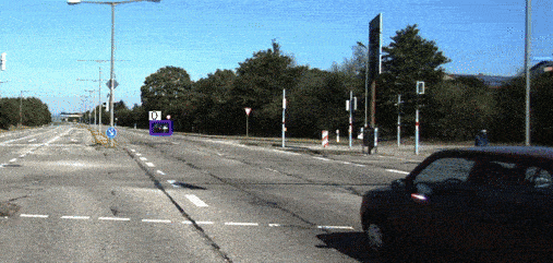
As shown, the tracker handles cars entering the scene reasonably well. However, a closer look reveals two specific problems:

• Missing track for the big truck: The object detector fails to identify the truck, which means no track is created for it. A natural next step would be to explore alternative object detection algorithms. Object detection is a critical and open area of research. In fact, KITTI also offers an object detection challenge to benchmark such algorithms.

• Occlusion of the yellow car: Towards the end of the sequence, a yellow car is trying to enter the highway. It gets occluded by other vehicles. We see that a track with ID 21 is created, but it is dropped due to occlusion, and another track with ID 23 is created a few frames later. As stated before, occlusion remains a critical issue in camera-based object tracking. Many SOTA algorithms address this problem using various approaches. For example, Observation-Centric SORT is an extension of SORT that specifically tackles occlusion. Exploring such solutions could be a valuable next step.